Parallel Computation and Memory Management
The calculation of the p-values of the \(\Lambda\)-motifs demands computation power as well as working memory which grow quickly with the number of nodes. To address this problem, the calculation is split into chunks and the Python multiprocessing package is used.
Parallel Computation
By default the computation is performed in parallel using the multiprocessing packge. The number
of parallel processes depends on the number of CPUs of the work station and is
defined by the variable num_procs in the method BiCM.get_pvalues_q()
(see API).
If the calculation should not be performed in parallel, use:
>>> cm.lambda_motifs(<bool>, parallel=False)
instead of:
>>> cm.lambda_motifs(<bool>)
Memory Management
In order to calculate the p-values, information on the \(\Lambda\)-motifs and their probabilities has to be kept in the working memory. This can lead to memory allocation errors for large networks due to limited resources. To avoid this problem, the total number of p-value operations is split into chunks which are processed sequentially. The number of chunks can be defined when calling the motif function:
>>> cm.lambda_motifs(<bool>, num_chunks=<number_of_chunks>)
The default value is num_chunks = 4. As an example, for \(N\) nodes in a
bipartite layer, \(\binom{N}{2}\) p-values have to be computed. If
num_chunks = 4, each chunk processes therefore about
\(\frac{1}{4}\binom{N}{2}\) p-values in parallel.
Note
Increasing num_chunks decreases the required working memory, but leads
to longer processing times. For \(N \leq 15\), num_chunks = 1 by
default.
A Note on the Output Format
A layer composed of \(N\) vertices requires the computation of \(\binom{N}{2}\) p-values to assess the node similarities. They are saved in the output file as a one-dimensional array when running the method :func:`BiCM.get_pvalues_q``cm.lambda_motifs`. However, a more intuitive matrix representation can be easily recovered using some helper functions, since each element in the array can be mapped on an element in the matrix and vice versa.
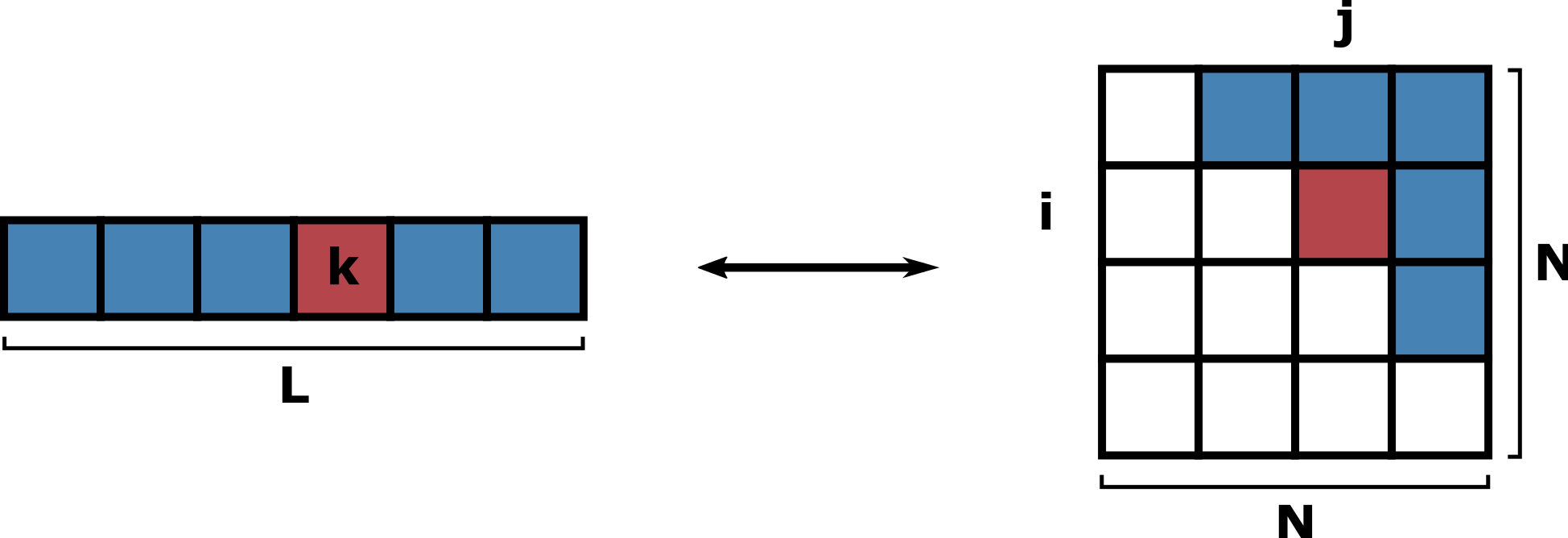
Figure 1: Mapping of the one-dimensional array of length \(L\) onto a square matrix of dimension \(N \times N\). Note that the matrix is symmetric.
Let’s consider an array of length \(L\) as shown in Figure 1. The dimension \(N\) of the matrix, i.e. the number of nodes in the original bipartite network layer, can be obtained as:
>>> N = cm.flat2triumat_dim(L)
To convert an array index k to the corresponding matrix index couple (i,
j) in the upper triangular part, use:
>>> (i, j) = cm.flat2triumat_idx(k, N)
Note
As illustrated in Figure 1, the output array contains the upper triangular part of the symmetric square matrix, excluding the diagonal. Thus
- \(k \in [0, \ldots, N (N - 1) / 2 - 1]\)
- \(i \in [0,\ldots, N - 1]\)
- \(j \in [i + 1,\ldots, N - 1]\)
The inverse operations are given by:
>>> L = cm.triumat2flat_dim(N)
>>> k = cm.triumat2flat_idx(i, j, N)