Tutorial¶

The tutorial will take you step by step from the biadjacency matrix of a real-data network to the calculation of the p-values. Our example bipartite network will be the following:

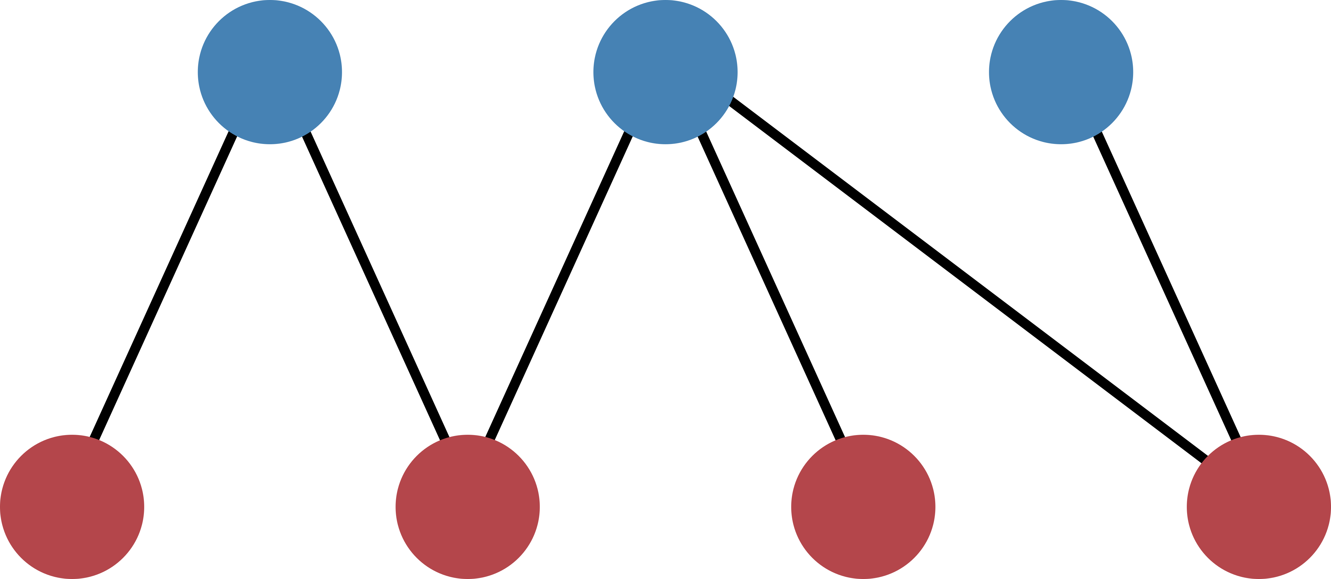
Figure 1: Example network.

The structure of the network can be captured in a biadjacency matrix. In our case, the matrix is

\[\begin{split}\left[ \begin{matrix} 1 & 1 & 0 & 0 \\ 0 & 1 & 1 & 1 \\ 0 & 0 & 0 & 1 \end{matrix} \right]\end{split}\]

Note that the nodes of the top layer are ordered along the rows and the nodes of the bottom layer along columns. In the bicm module, the two layers are identified by the boolean values True for the row-nodes and False for the column-nodes. In our example image, the row-nodes are colored in blue (True, top layer) and the column-nodes in red (False, bottom layer).

The bicm module encompasses essentially two steps for the validation of node similarities in bipartite networks:

Given a binary input matrix capturing the network structure, create the biadjacency matrix of the BiCM null model.
Calculate the p-values of the node similarities for the same bipartite layer.

Subsequently, a multiple hypothesis testing of the p-values can be performed. The statistically validated node similarities give rise to a unbiased monopartite projection of the original bipartite network, as illustrated in [Saracco2017].

For more detailed explanations of the methods, please refer to [Saracco2017].

Getting started¶

We start by importing the necessary modules:

>>> import numpy as np
>>> from src.bicm import BiCM

The biadjacency matrix of our network can be captured by the two-dimensional NumPy array mat

>>> mat = np.array([[1, 1, 0, 0], [0, 1, 1, 1], [0, 0, 0, 1]])

and we initialize the Bipartite Configuration Model with:

>>> cm = BiCM(bin_mat=mat)

Biadjacency matrix¶

In order to obtain the individual link probabilities between the top and the bottom layer, which are captured by the biadjacency matrix of the BiCM null model, a log-likelihood maximization problem has to be solved, as described in [Saracco2017]. This can be done automatically by running

>>> cm.make_bicm()

In our example graph, the BiCM biadjacency matrix should be:

>>> print cm.adj_matrix
[[ 0.29433408  0.70566592  0.29433408  0.70566592]
 [ 0.60283296  0.89716704  0.60283296  0.89716704]
 [ 0.10283296  0.39716704  0.10283296  0.39716704]]

Note that make_bicm outputs a status message in the console of the form:

Solver successful: True
The solution converged.

The message informs the user whether the underlying numerical solver has successfully converged to a solution and prints its status message.

We can check the maximal degree difference between the input network and the BiCM model by running:

>>> cm.print_max_degree_differences()

Note

The function make_bicm uses the scipy.optimize.root routine of the SciPy package to solve the maximization problem. It accepts the same arguments as scipy.optimize.root except for fun and args, which are specified in our problem. This means that the user has full control over the selection of a solver, the initial conditions, tolerance, etc.

As a matter of fact, in some situations it may happen that the function call make_bicm(), which uses default arguments, does not converge to a solution. In that case, the console will report Solver successful: False together with the status message returned by the numerical solver.

If this happens, the user should try different solvers, such as least-squares and/or different initial conditions or tolerance values.

Please consult the scipy.optimize.root documentation with a list of possible solvers and the description of the function make_bicm in the API.

After having successfully obtained the biadjacency matrix, we could save it in the file <filename> with

>>> cm.save_biadjacency(filename=<filename>, delim='\t')

The default delimiter is \t and does not have to be specified in the line above. Other delimiters such as , or ; work fine as well. The matrix can either be saved as a human-readable .csv or as a binary NumPy .npy file, see save_biadjacency() in the API. In the latter case, we would run:

>>> cm.save_biadjacency(filename=<filename>, binary=True)

If binary == True, the file ending .npy is appended automatically.

P-values¶

Each entry in the biadjacency matrix of the null model corresponds to the probability of observing a link between the corresponding row- and column-nodes. If we take two nodes of the same layer, we can count the number of common neighbors that they share in the original input network and calculate the probability of observing the same or more common neighbors according to the BiCM [Saracco2017]. This corresponds to calculating the p-values for a right-sided hypothesis testing.

The number of common neighbors can be described in terms of \(\Lambda\)-motifs [Saracco2017], as shown in Figure 2.

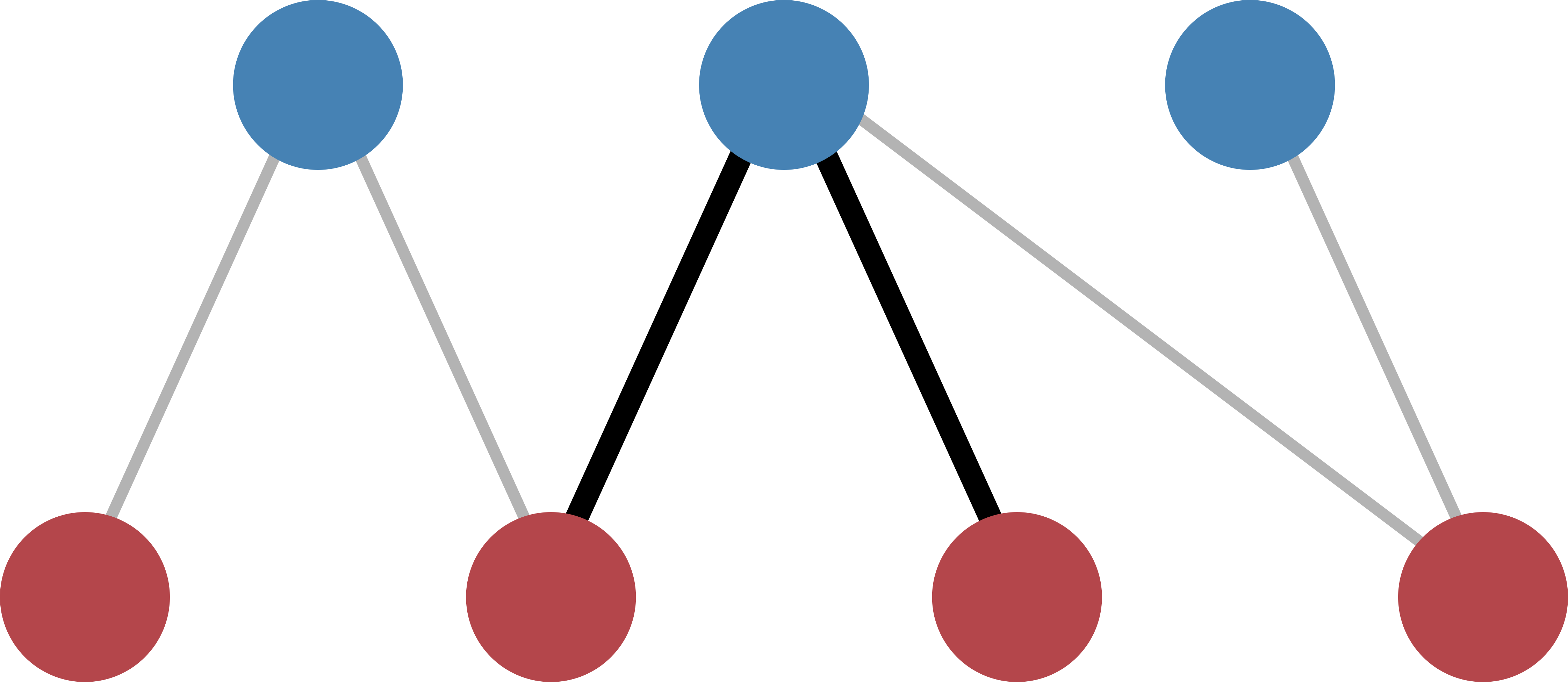
Figure 2: Illustration of a \(\Lambda\)-motif between the two central red nodes.

The calculation of the p-values is computationally intensive and should be performed in parallel, see Parallel Computation and Memory Management for details. It can be executed by simply running

>>> cm.lambda_motifs(<bool>, filename=<filename>)

where <bool> is either True of False depending on whether we want to address the similarities of the row- or column-nodes, respectively. The results are written to <filename>. By default, the file is a binary NumPy file to reduce disk space, and the format suffix .npy is appended. If the file should be saved in a human-readable .csv format, we need to provide an appropriate name ending with .csv and use:

>>> cm.lambda_motifs(<bool>, filename=<filename>, delim='\t', binary=False)

Again the default delimiter is \t.

Note

The p-values are saved as a one-dimensional array with index \(k \in \left[0, \ldots, \binom{N}{2} - 1\right]\) for a bipartite layer of \(N\) nodes. Please check the section A Note on the Output Format for details regarding the indexing.

Having calculated the p-values, it is possible to perform a multiple hypothesis testing of the node similarities and to obtain an unbiased monopartite projection of the original bipartite network. In the projection, only statistically significant edges are kept.

For further information on the post-processing and the monopartite projections, please refer to [Saracco2017].